Getting Started#
scphylo is a comprehensive Python toolkit designed to unify single-cell tumor phylogeny inference methods. It addresses the lack of standardization in the field by providing a cohesive interface for data processing, tree reconstruction, and visualization.
By streamlining these tasks, scphylo empowers researchers to easily utilize complex inference methods, ensuring reproducible benchmarking and democratizing access to advanced computational oncology tools.
Installation#
pip install scphylo-tools
Workflow Overview#
scphylo is organized into modular components that cater to different stages of the phylogenetic analysis workflow:
Module |
Description |
|---|---|
``scphylo.io`` |
Data Management: Unified interface for reading and writing genotype and read-count matrices. Handles format inconsistencies between tools. |
``scphylo.pp`` |
Preprocessing: Utilities to mitigate noise (ADO, false positives) and sparsity. Includes filtering, matrix optimization (bifiltering), and consensus aggregation. |
``scphylo.tl`` |
Inference: A unified solver interface wrapping state-of-the-art algorithms (e.g., SCITE, PhISCS, HUNTRESS) using standard Python syntax. |
``scphylo.pl`` |
Visualization: Tools to render annotated phylogenetic trees and sorted genotype heatmaps using Matplotlib and Graphviz. |
``scphylo.datasets`` |
Datasets: Access to curated, high-impact single-cell tumor datasets (e.g., Leukemia, Breast Cancer, Melanoma). |
``scphylo.ul`` |
Utilities: Metrics for tree evaluation (Robinson-Foulds, MP3) and a simulation engine for generating synthetic tumor phylogenies. |
Quick Start Example#
This guide demonstrates how to load a dataset, preprocess it, infer a tumor phylogeny, and visualize the results.
1. Import scphylo#
[ ]:
import scphylo as scp

scp.settings.verbosity = 3
scp.logg.print_version()
Running scphylo 0.0.5 (python 3.12.12) on 2025-12-24 20:16.
2. Load a Dataset#
scphylo provides easy access to published datasets. Here, we load a dataset from a melanoma cancer study.
[ ]:
adata = scp.datasets.example()
print(adata)
print("\nCells info:\n", adata.obs.head())
print("\nMutations info:\n", adata.var.head())
AnnData object with n_obs × n_vars = 83 × 452
    obs: 'group', 'subclone_color', 'Axl', 'Erbb3', 'Mitf', 'MPS'
    var: 'CHROM', 'POS', 'REF', 'ALT', 'START', 'END', 'Allele', 'Annotation', 'Gene_Name', 'Transcript_BioType', 'HGVS.c', 'HGVS.p'
    layers: 'genotype', 'mutant', 'total'

Cells info:
       group subclone_color   Axl  Erbb3  Mitf    MPS
cell
C15_1   C15        #B9D7ED 6.328  0.000 0.000 -0.728
C15_2   C15        #B9D7ED 6.978  3.604 4.067  0.170
C15_3   C15        #B9D7ED 7.418  5.479 5.460 -1.208
C15_4   C15        #B9D7ED 8.462  4.725 2.711 -2.572
C15_5   C15        #B9D7ED 6.884  6.314 0.000 -0.621

Mutations info:
            CHROM       POS REF    ALT     START       END Allele          Annotation Gene_Name  \
mutation
mutation_1  chr1  15815968   A  ['G']  15815968  15815968      G    missense_variant     Terf1
mutation_2  chr1  37396158   G  ['A']  37396158  37396158      A  synonymous_variant    Inpp4a
mutation_3  chr1  38045805   T  ['C']  38045805  38045805      C    missense_variant     Eif5b
mutation_4  chr1  51071476   G  ['A']  51071476  51071476      A    missense_variant    Tmeff2
mutation_5  chr1  54997173   A  ['G']  54997173  54997173      G    missense_variant     Sf3b1

           Transcript_BioType     HGVS.c       HGVS.p
mutation
mutation_1     protein_coding   c.581A>G  p.Tyr194Cys
mutation_2     protein_coding  c.2622G>A  p.Val874Val
mutation_3     protein_coding  c.2732T>C  p.Val911Ala
mutation_4     protein_coding   c.448G>A  p.Gly150Ser
mutation_5     protein_coding  c.2740T>C  p.Phe914Leu
3. Preprocess the Data#
Real-world single-cell data often contains noise and missing values. We can filter out uninformative features and optimize the matrix.
[ ]:
scp.pp.filter_mut_vaf_greater_than_coverage_mutant_greater_than(
    adata, min_vaf=0.4, min_coverage_mutant=20, min_cells=2
)
scp.pp.filter_mut_reference_must_present_in_at_least(adata, min_cells=1)
scp.pp.filter_mut_mutant_must_present_in_at_least(adata, min_cells=2)
Matrix with n_obs × n_vars = 83 × 268
Matrix with n_obs × n_vars = 83 × 267
Matrix with n_obs × n_vars = 83 × 267
4. Infer Phylogeny#
Infer the evolutionary history using one of the supported solvers. scphylo wraps the complexity of input formatting and binary execution.
[ ]:
scp.pp.build_scmatrix(adata)
df_in = adata.to_df()
[ ]:
df_out = scp.tl.scistree(df_in, alpha=0.001, beta=0.2)
running ScisTree with alpha=0.001, beta=0.2
input -- size: 83x267
input -- 0: 9968#, 45.0%
input -- 1: 4020#, 18.1%
input -- NA: 8173#, 36.9%
input -- CF: False
output -- size: 83x267
output -- 0: 11308#, 51.0%
output -- 1: 10853#, 49.0%
output -- NA: 0#, 0.0%
output -- CF: True
output -- time: 59.0s (0:00:59.043201)
flips -- #0->1: 1881
flips -- #1->0: 27
flips -- #NA->0: 3194
flips -- #NA->1: 4979
rates -- FN: 0.320
rates -- FP: 0.00332758
rates -- NA: 0.369
score -- NLL: 4112.965352416734
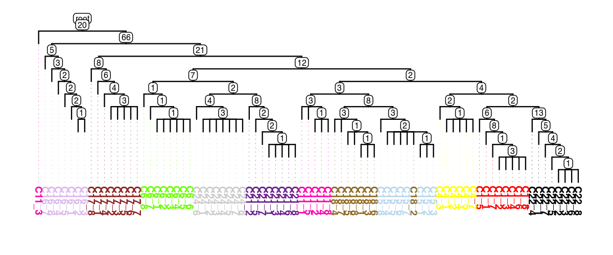
5. Visualize Results#
Visualize the inferred tree structure and the corresponding genotype heatmap.
[ ]:
tree = scp.ul.to_tree(df_out)
scp.pl.dendro_tree(
    tree,
    cell_info=adata.obs,
    label_color="subclone_color",
    width=1200,
    height=500,
    dpi=200,
)
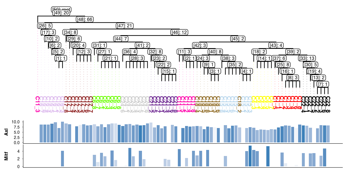
[ ]:
scp.pl.dendro_tree(
    tree,
    cell_info=adata.obs,
    label_color="subclone_color",
    width=1200,
    height=600,
    dpi=200,
    distance_labels_to_bottom=3,
    inner_node_type="both",
    inner_node_size=2,
    annotation=[
        ("bar", "Axl", "Erbb3", 0.2),
        ("bar", "Mitf", "Mitf", 0.2),
    ],
)
List of mutations branching at node with id [43]
[ ]:
mut_ids = tree.graph["mutation_list"][tree.graph["mutation_list"]["node_id"] == "[43]"]
adata.var.loc[mut_ids.index]
| CHROM | POS | REF | ALT | START | END | Allele | Annotation | Gene_Name | Transcript_BioType | HGVS.c | HGVS.p | |
|---|---|---|---|---|---|---|---|---|---|---|---|---|
| index | ||||||||||||
| mutation_162 | chr7 | 28042135 | A | ['C'] | 28042135 | 28042135 | C | missense_variant | Psmc4 | protein_coding | c.1109T>G | p.Ile370Ser |
| mutation_349 | chr13 | 103753116 | T | ['G'] | 103753116 | 103753116 | G | synonymous_variant | Srek1 | protein_coding | c.1039A>C | p.Arg347Arg |
| mutation_429 | chr19 | 4035556 | G | ['C'] | 4035556 | 4035556 | C | missense_variant | Gstp1 | protein_coding | c.550C>G | p.Leu184Val |
| mutation_8 | chr1 | 74287097 | T | ['G'] | 74287097 | 74287097 | G | missense_variant | Pnkd | protein_coding | c.242T>G | p.Ile81Ser |
[ ]: